About Electromyography

The nature of sEMG recordings

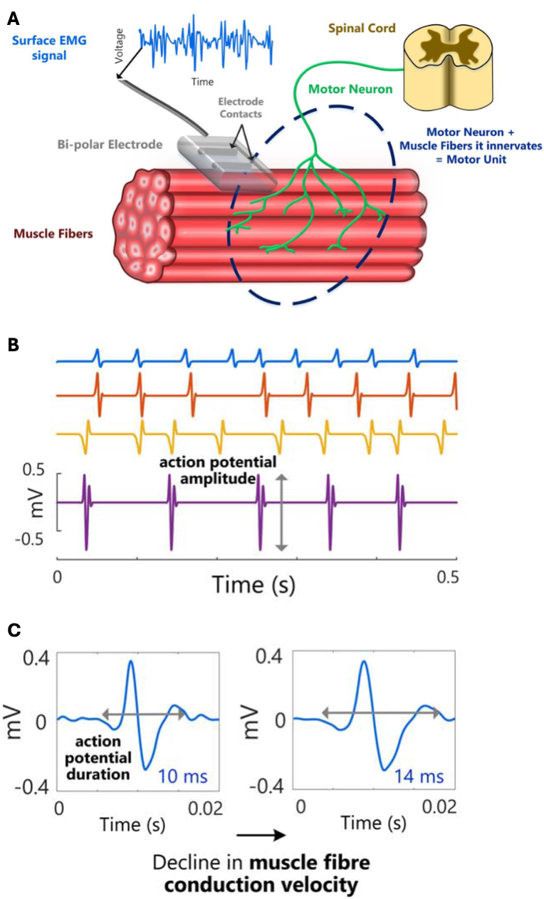
Surface electromyography (sEMG) is a non-invasive technique that quantifies muscle activity by recording voltages at the skin overlying a muscle, as illustrated in Figure 1A. Voluntary movement arises from muscle contraction: motoneuron discharges activate groups of fibers (motor units), generating motor‐unit action potentials (MUAPs) that propagate along the fibers with a characteristic conduction velocity, as illustrated in Figure 1B-C.

Each discharge produces a brief force twitch; the superposition of many twitches over time yields sustained force for actions such as lifting or smiling (McManus, De Vito, & Lowery, 2020; De Luca, 2008). sEMG captures the resulting voltage time series from which quantitative features are extracted (Fridlund & Cacioppo, 1986).

Figure 1. (A) Example sEMG signal recording. (B) Motor unit action potential, and (C) Relationship between MUAP duration and muscle fibre conduction velocity. Adapted from McManus, De Vito, & Lowery, 2020.

EMG Signal Processing Overview

EMG signal processing converts raw voltage time series into interpretable representations and features. Two complementary views are central:

• Time domain shows amplitude versus time. It reveals transients, drift, motion artefacts, and waveform shape. This view is used to select passband edges and to confirm that preprocessing preserves morphology.

• Frequency domain summarizes power versus frequency (power spectral density; PSD). It exposes mains peaks and harmonics and characterizes the bandwidth of physiological activity. This view is used to set notch parameters (f0, Q) and to verify that the chosen passband matches the target physiology.

Figure 2 illustrates how these views work together during preprocessing. Panels A–D show the same signal segment before and after filtering in both the time and frequency domains.

Figure 2. Time and PSD views of the same sEMG segment. A) Raw time-series shows drift and periodic contamination. B) Raw PSD shows mains peaks and overall bandwidth. C) After notch and bandpass filtering, the time-series is cleaned; the rectified-RMS envelope (thin line) provides amplitude over time. D) Filtered PSD confirms removal of mains peaks and a defined passband.

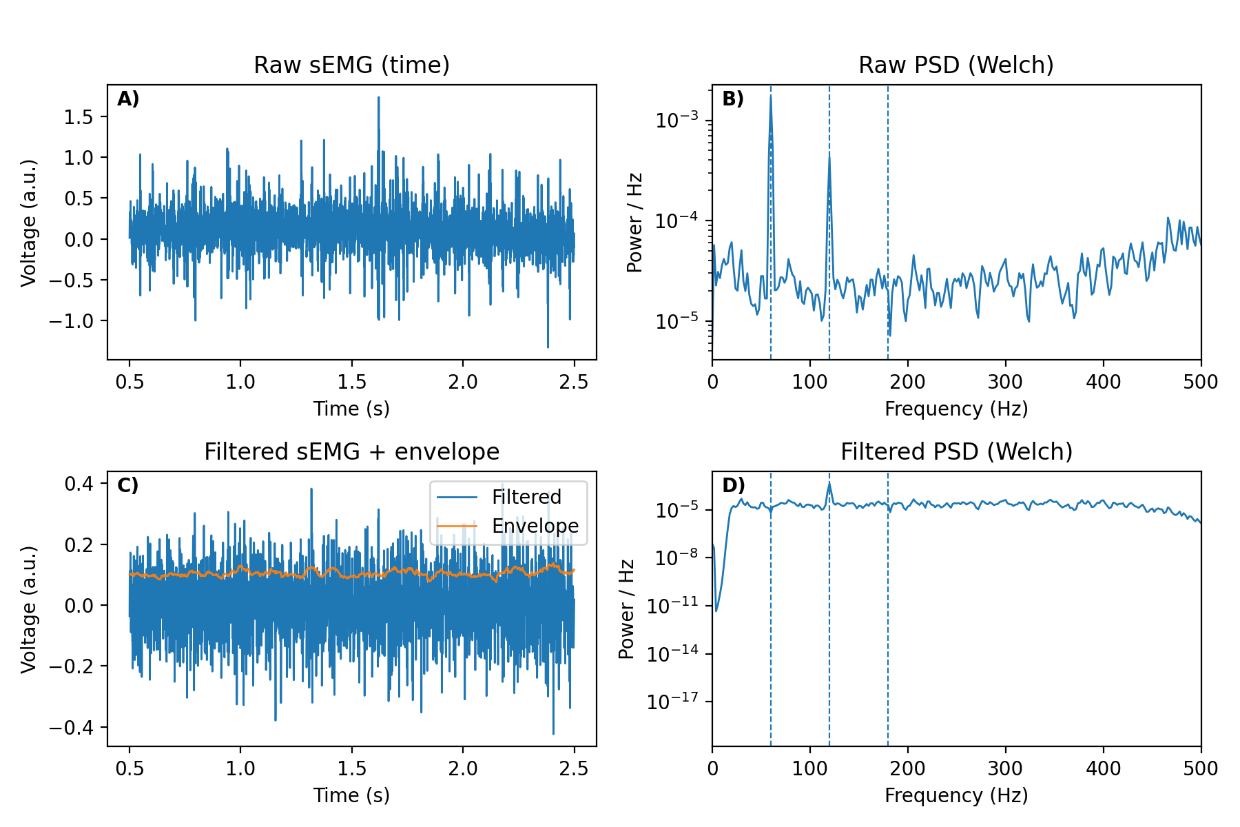
How to read Figure 2

• A) Raw time series (time domain). Inspect for low-frequency drift, motion artefacts, clipping, and bursts. Use this panel to choose passband edges and to ensure filters do not distort salient events.

• B) Raw PSD (frequency domain). Identify mains peaks (50/60 Hz and harmonics) and estimate the physiological band that contains most power. Use this panel to set notch parameters (f0, Q) and to motivate the bandpass.

• C) Filtered time series with envelope. After applying notch and bandpass filters, verify that drift and hum are removed while event shape is preserved. The rectified-RMS envelope aids visualization and feature extraction.

• D) Filtered PSD. Confirm that mains peaks are suppressed and that the passband matches the intended physiological range.

Together, the time- and frequency-domain views provide cross-checks: choose and verify passband edges in time; select and verify notch parameters in frequency.

Domains of EMG Features

EMG features are commonly organized into:

• Time-domain features quantify amplitude and variability over time (e.g., RMS, MAV, iEMG, waveform length, Willison amplitude).

• Frequency-domain features quantify spectral location, spread, and shape (e.g., mean frequency, median frequency, bandwidth, spectral entropy).

• Time–frequency features track spectral content over time (e.g., windowed spectra or wavelets). EMGFlow emphasizes established time- and frequency-domain features; time–frequency analyses can be derived from the same PSD and envelope primitives when needed (see, e.g., Chowdhury et al., 2013).

EMGFlow Definitions

Signal

In EMGFlow, signals are represented as Pandas DataFrames, typically read from CSV files. Standard EMGFlow DataFrames include:

• A Time column recording elapsed time (seconds).
• Additional columns for EMG signal magnitudes from each electrode.

Units for signal magnitudes should be consistent within each file to ensure valid comparisons. The Time column is primarily for visualization and is not essential for computations if the sampling rate is known. Any column labelled Time is treated as a time reference and may be ignored during calculations.

Sampling Rate

The sampling rate (sampling_rate) defines how many samples are recorded per second. When Time is absent or irregular, the sampling rate specifies the temporal spacing for analysis.

Power Spectral Density (PSD)

A PSD DataFrame represents the frequency-domain view of an EMG signal obtained via Fourier analysis. EMGFlow computes PSDs using Welch’s method—overlapped, windowed averaging, typically with a Hann window—to produce stable spectral estimates that complement the time-series view (LDS Group, 2003).

Sources

• Chowdhury, R. H., Reaz, M. B. I., Ali, M. A. B. M., Bakar, A. A. A., Chellappan, K., & Chang, T. G. (2013). Surface Electromyography Signal Processing and Classification Techniques. Sensors, 13(9), Article 9. https://doi.org/10.3390/s130912431
• De Luca, C. J. (2008). The practicum of electromyography.
• Fridlund, A. J., & Cacioppo, J. T. (1986). Guidelines for human electromyographic research. Psychophysiology, 23(5), 567–589.
• Lindström, L., Kadefors, R., & Petersen, I. (1977). An electromyographic index for localized muscle fatigue. Journal of Applied Physiology, 43(4), 750–754. https://doi.org/10.1152/jappl.1977.43.4.750
• McManus, L., De Vito, G., & Lowery, M. M. (2020). Analysis and interpretation of surface EMG signals. Frontiers in Physiology, 11, 1039.
• LDS Group. (2003). Understanding FFT Windows. Application Note ANO14. https://www.egr.msu.edu/classes/me451/me451_labs/Fall_2013/Understanding_FFT_Windows.pdf